
- Using APOGEE Spectra
- How should I convert the vacuum wavelengths to air?
- Why are there gaps in APOGEE spectra?
- What are the uncertainties on APOGEE spectra?
- What might be affecting my spectra?
- Imperfect Subtraction of Night Sky Lines
- Bad Pixels/Missing Regions
- Ghosts
- Fiber Cross Talk
- Persistence in the “Blue” Detector
- Using BOSS Spectra
- What is the resolution of the BOSS spectra?
- Is the spectrophotometric calibration as good in the FPS era as in the plate era?
- Why are there weird features in my spectrum?
- Jumps in the Spectrum
- The Scoop
- The Wiggles (no, not those Wiggles)
- What else might be affecting my spectrum?
- Poor sky subtraction
- Poor wavelength calibration
Milky Way Mapper wavelengths are in vacuum, not air.
Using APOGEE Spectra
How should I convert the vacuum wavelengths to air?
The wavelength calibration of the APOGEE data is done using vacuum wavelengths. However, the wavelengths of atomic transitions in the optical and infrared are usually quoted at standard temperature and pressure (S.T.P.); this is how the CRC Handbook of Chemistry and Physics lists them for transitions redward of 2000 Ångströms. Thus, spectral lines associated with specific atomic transitions may require converting the SDSS data to the equivalent values at S.T.P. For APOGEE data, the conversion from Ciddor (Applied Optics, Vol 35, p 1566, 1996) has been employed to convert between vacuum and air wavelengths. For a vacuum wavelength (VAC) in Ångströms, convert to air wavelength (AIR) using the equation:
Why are there gaps in APOGEE spectra?
The spectra are recorded onto three different detectors (“chips”). While the overall coverage ranges from 1.514 to 1.696 microns, there are small gaps between the detectors, which result in gaps in the wavelength coverage. While all of the spectra lie in the infrared H– band, sometimes the chips are referred to as the “blue”, “green”, and “red” chips, going from the shorter wavelengths to longer wavelengths. Data products refer to the separate chips as chips “a”, “b”, and “c”, in the order in which they are read out. As it turns out, the “red” chip is the first one to read out, so this nomenclature is in reverse wavelength order. The following table explains the terminology.
| chip | name | start wavelength | end wavelength | central dispersion |
|---|---|---|---|---|
| a | “red” | 1.647 μm | 1.696 μm | -0.236 A/pix |
| b | “green” | 1.585 μm | 1.644 μm | -0.283 A/pix |
| c | “blue” | 1.514 μm | 1.581 μm | -0.326 A/pix |
Note that the starting and ending wavelengths vary slightly from fiber to fiber because of variations of their placement along the instrument pseudo-slit. The dispersion varies with wavelength, and, to a lesser extent, by fiber.
For ease in analysis, all of the spectra are rebinned to the same dispersion and wavelength axis such that “chip gaps” fall in the same place for all spectra.
What are the uncertainties on APOGEE spectra?
All APOGEE spectra include an array of uncertainties (“errors”) for each pixel; these are given as the standard deviation of the flux values. These uncertainties are initially calculated from the raw pixel data based on the inherent properties of the detectors (gain and readout noise). These are then propagated into the uncertainties for subsequent data products.
However, in downstream spectral products, data for any given pixel may have been derived from some combination of pixels in the raw data, and data from any individual raw pixel may contribute to more than one pixel in the combined spectra. As a result, there may be correlated errors between pixels and can occur even in visit spectra because these are the combination of two dithered observations. If the dithers are spaced by 0.5 pixels exactly, then the spectral combination software interleaves the two dithered exposures. Still, if the dithers are even slightly imperfect (as they generally are), any pixel in the combined well-sampled spectrum will have contributions from multiple raw pixels. For the visit-combined apStar/asStar spectra, the pixels have inputs from multiple raw pixels, because the apStar/asStar spectra are RV-corrected and resampled onto a standard wavelength grid. Although the uncertainties are propagated into the apVisit/asVisit and apStar/asStar spectra, this propagation ignores the correlation of uncertainties that result from having processed pixels that are derived from multiple raw pixels.
Multiple observations of selected targets have been used to estimate empirical uncertainties, and these demonstrate that, for most targets, the calculated uncertainties are reasonable, i.e., the scatter from observation to observation is comparable to the estimated uncertainty for each observation. However, for very bright targets, the calculated uncertainties are almost certainly underestimated because systematic uncertainties most likely limit the accuracy of these data from the data processing and in the calibration data products. These have not yet been fully quantified, but we expect an uncertainty “floor” at the 0.5% level, i.e., a maximum S/N of ~200. Such a floor has not been set in the spectrum uncertainty arrays, and so, users should be aware that there is a likely maximum S/N~200.
What might be affecting my spectra?
Imperfect Subtraction of Night Sky Lines
The night sky lines (i.e., “airglow”), primarily from OH emission in the Earth’s atmosphere, can be extremely bright. The sky emission is removed from the science spectra using the combination of the emission from sky fibers at sky positions near that of the target. However, this subtraction is almost always imperfect for two reasons. First, the sky spectrum has to be wavelength-shifted to match the science spectra; this occurs because the fibers have different locations along the pseudo-slit. Second, the line spread function (LSF) varies by fiber due to changes in image quality across the field-of-view. Because the night skylines are so bright, even small fractional variations due to these issues can cause the subtraction to be very noticeably imperfect; thus, most skylines are either under- or over-subtracted.
Note that, even if the airglow subtraction were perfect, the area of the spectrum “under” the skylines would be of significantly lower signal-to-noise, due to the substantial Poisson contribution from the bright lines.
The imperfect night sky line subtraction does have the unfortunate result of making the APOGEE spectra appear a bit “ugly” to a quick, casual inspection. The APOGEE data products (e.g., apVisit/asVisit and apStar/asStar files) include a record of the sky spectrum that was subtracted, and it is possible to use this as a guide for recognizing pixels that are likely to be affected by imperfect sky subtraction.
Bad Pixels/Missing Regions
The IR detectors used for APOGEE are not cosmetically perfect. Small regions of each chip are bad, and there are a significant number of individual bad or “hot” pixels. These are flagged during the data processing and can lead to bad or missing regions in any given spectrum. Because visit spectra are combined from multiple individual dithered spectra, a single bad pixel can propagate into multiple pixels in the visit-combined spectra. In combination with the poorly subtracted skylines, these bad pixels can have the effect of making individual visit spectra look rather “ugly.” The mask arrays can be used to identify the cause of most bad pixels.
Because any given star will typically not use the same fiber for different visits, combined spectra generally look somewhat cleaner, especially if the observed radial velocity (including differences in barycentric RV) of a target differs significantly from visit-to-visit. However, even if the combined spectra do not have regions with missing data, there may be regions where the noise level is elevated if that portion of the spectrum landed on a bad region of one of the arrays in one or more of its visits.
Ghosts
The use of VPH gratings results in the production of some “ghosts” on the 2-D images. The most prominent of these is the “Littrow ghost,” which for the APOGEE data falls somewhere in the wavelength region 1.605 ± 10 microns, depending on the fiber (e.g. Wilson et al. 2019).
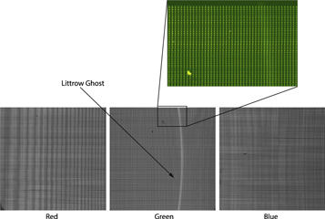
Littrow ghost from Wilson et al. 2019
The amplitude of the ghost depends on the brightness of other stars in the field, so it does not always contribute a significant amount of flux. Pixels possibly affected by the “Littrow ghost” are flagged with the LITTROW_GHOST bit in the APOGEE_PIXMASK bitmask.
Fiber Cross Talk
The spacing of adjacent spectra is ~ 6.5 pixels (as measured between adjacent PSF peaks) to pack the spectra of as many stars as possible across the APOGEE detectors. Therefore, the wings of the PSF overlap slightly between neighboring spectra, and the effect is particularly apparent if an object is located adjacent to a much brighter object.
In APOGEE-1 and -2, the targets on each plate are sorted into three brightness categories — bright (B), medium (M), and faint (F) — and these categories are placed along the pseudo-slit (and hence, on the detectors) in the order FMBBMF FMBBMF. This fiber management was not done in MWM.
The extraction portion of the data reduction pipeline accounts for contributions of light from the two neighboring spectra for each target. The effectiveness of this extraction depends on our knowledge of the amplitude of the wings of the light distribution. In cases where adjacent targets are significantly brighter than a given object, small inaccuracies in the PSF model may lead to significant errors in the extraction of the spectrum.
For each visit, a bit is set in the APOGEE_STARFLAG bitmask if an adjacent object is more than 100 times brighter than the star itself (VERY_BRIGHT_NEIGHBOR) or more than 10 times brighter (BRIGHT_NEIGHBOR). The former case, which is rare, is automatically considered as a bad spectrum and will not be included in the combined spectrum.
Persistence in the “Blue” Detector
Some areas of the detectors used in the APOGEE northern instrument suffer from a problem referred to as “super-persistence.” In these locations on the detector, previous exposure to light causes a glow in subsequent images that can be substantial and last for a significant amount of time. The problem is most severe on about 1/3 of the “blue” chip, i.e., the chip that records wavelengths between 1.514 and 1.581 microns. Due to the chip orientation, this full wavelength region may be impacted for all objects in this part of the chip (~1/3). There are also regions in the “green” chip that are affected by a lower level of super-persistence, but these regions are less clearly defined by fiber number or wavelength.
After the completion of the APOGEE-1 survey in summer 2014, the instrument was opened, and the blue detector, which had the worst impact from super-persistence, was replaced with a detector with better performance. While this will mitigate the effects of super-persistence for data taken after summer 2014, DR16 includes data taken from before this date as well.
The impact of super-persistence for a given object is dependent on (1) the prior exposure history and (2) the brightness of the current target. The fiber management system described in the Fiber Cross Talk section provides some level of mitigation. Grouping the fibers by target brightness makes it relatively uncommon for a faint target to be observed through a fiber that was previously placed on a bright target. However, because the magnitude ranges that define these categories are broad, there can still be cases where faint targets follow relatively brighter ones. Also, calibration flat field exposures are taken between every plate to map the distribution of light between fibers and to measure the fiber-to-fiber throughput variations. These roughly evenly-illuminated frames are sufficient to give rise to some super-persistence.
Superpersistence is a complex phenomenon. In DR13/DR14, we attempted to implement a first-order super-persistence correction, based on some calibration data that were obtained, and scaling the results to try to match persistence observed in dark frames taken before most of the science exposures. We also implemented a scheme in which pixels affected by persistence are assigned a lower weight when different visits are combined. Additional description of how this problem is addressed is available in Holtzman et al. (2018). We implemented the same procedure for DR17.
The effect of super-persistence can be significant and is easily noticed: the flux levels in the region of the spectrum affected can be enhanced by tens of percent or more. This enhancement is likely to have some wavelength dependence meaning that spectral features may be distorted. However, depending on the brightness of the target and the preceding ones, it is not guaranteed that the spectra are adversely affected at a significant level, so we do not flag all data that falls within the super-persistence region as bad by default.
In the data reduction pipeline, we flag all pixels in the regions where significant superperstence is known to occur in the APOGEE_PIXMASK bitmask using three different flags corresponding to the level of the effect: PERSIST_HIGH, PERSIST_MED, and PERSIST_LOW. In addition, we have a visit level flag, APOGEE_STARFLAG, for each object, with bits that get set when a significant number of pixels (>20%) in the spectrum are affected, which are again split into categories of PERSIST_HIGH, PERSIST_MED, and PERSIST_LOW. In addition, we look for evidence in the spectra of a “jump” in flux between the “green” and the “blue” chips, and if this is present at an easily recognized level, we set a flag PERSIST_JUMP_HIGH or PERSIST_JUMP_LOW if the “blue” portion of the spectrum seems abnormally high or abnormally low (the latter could occur, e.g., if a sky fiber from a region affected by superpersistence is used for sky subtraction, although the pipeline takes some steps to try to avoid this occurrence).
In the combined spectra, star level flags are provided that are bitwise AND and bitwise OR combinations of the visit APOGEE_STARFLAG flags to indicate whether a given object was marked as having a significant number of pixels in the super-persistence region in all or any of the visit spectra comprising the combination. Starting in DR13, a scheme was implemented in which pixels affected by super-persistence are given inflated uncertainties to reduce their impact on the combined spectra. For those stars where some visits were impacted by super-persistence, and others were not, the random uncertainties are larger because those visits affected by the super-persistence are essentially ignored. For stars in which all visits are impacted by persistence, this has the effect of giving the persistence-affected wavelengths less weight in the ASPCAP fitting than pixels at other wavelengths.
As noted in Holtzman et al. (2015), the effects of persistence can be seen in some of the individual element abundances for the DR12 data. While this may be true for some objects in the current data release, comparison of results for stars unaffected by persistence to those affected by persistence in all visits suggests that the down-weighting scheme has helped significantly to mitigate persistence effects. The stars most likely to still be impacted are those that are the faintest stars or those with weak absorption features. Additional discussion on these issues relevant to the DR17 reductions can be found in Holtzman et al. (2018).
Using BOSS Spectra
What is the resolution of the BOSS spectra?
The resolution of the BOSS spectrographs varies from R~1220 blueward of 3800Å to R~1550-2550 redward of 4900Å (see Table 3 in Smee et al. 2013).
Is the spectrophotometric calibration as good in the FPS era as in the plate era?
Spectrophotometry is an ongoing issue in SDSS-V, and significant effort is being made to improve it. FPS observations between MJD=59635 (Feb 25 2022, start of FPS ops) and MJD=59732 (Jun 2 2022) have poorer spectrophotometry as we worked to improve our knowledge of fiber positions. FPS observations starting on MJD=59733 (Jun 3 2022) have significantly improved spectrophotometry that is similar to that of SDSS plate spectroscopy.
Medan et al. 2025 discuss the issues with spectrophotometry in the FPS era, where fiber positioning errors, atmospheric dispersion, and deliberate offset pointings make applying corrections tricky. If the true positions of the fibers, for example, are taken into account, the SEDs can be corrected for better spectrophotometric accuracy.
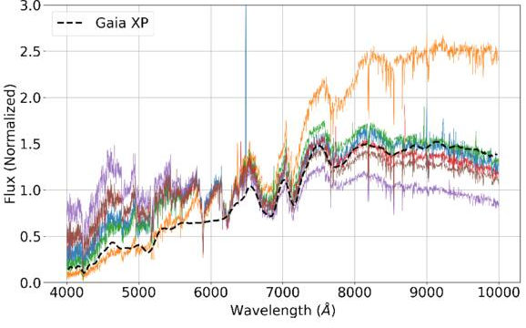
Example from Medan et al. 2025 of an obvious example of spectrophotometric issues. The colored lines show the same M dwarf after the standard flux calibration routine. The obviously different shapes of the SED are cause for concern.
Fries et al. 2023 give an example of improving the spectrophotometry using narrow emission lines in AGN spectra that are known not to vary on ~years long timescales. We are also exploring the use of Gaia XP spectra for the brighter stellar targets.
Why are there weird features in my spectrum?
Tom Dwelly and others have identified a number of ways in which BOSS spectra can have unexpected features. The causes for these are not always known, but if you see such a feature, it is likely to be non-astrophysical in origin.
Jumps in the Spectrum
If you see a jump around 5800Å, this means the spectra from the red and blue arms have been poorly joined. The BOSS pipeline handles the blue and red spectra independently until after flux calibrations, when they are combined using a weighted mean. If the spectrophotometric calibration, or trace, or flatfielding has failed for the spectrum from one arm, you can end up with a very interesting-looking spectrum.
Behold a case where the blue and red spectrum have been poorly joined. (Figure by Tom Dwelly)
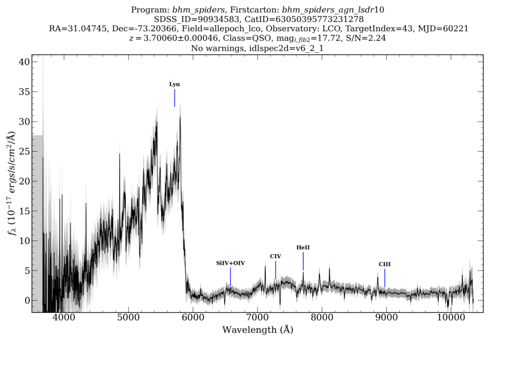
Some LCO BOSS spectra show a jump around 8000Å; the cause of this is not known. It can confuse the BOSS pipeline if it is mistaken for e.g., the Balmer break.
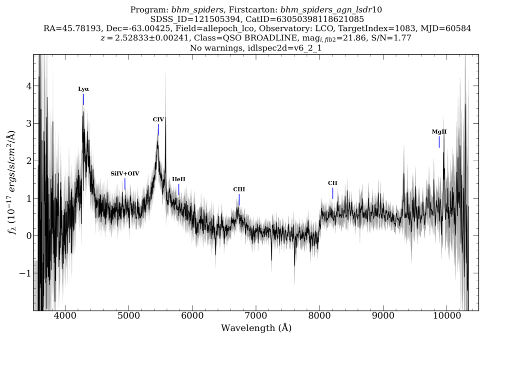
LCO spectra sometimes show an unexpected feature at 8000Å. (Figure from Tom Dwelly)
The Scoop
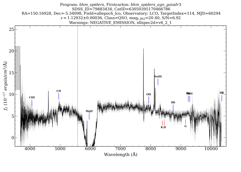
Spectra for objects that we expect to look fairly flat in the continuum exhibit a broad ‘scoop’ feature. Possibly associated with the 8000Å step. (Figure from Tom Dwelly)
The Wiggles (no, not those Wiggles)
These are prominent oscillations in the extracted spectrum, possibly caused by tracing/extraction issues.
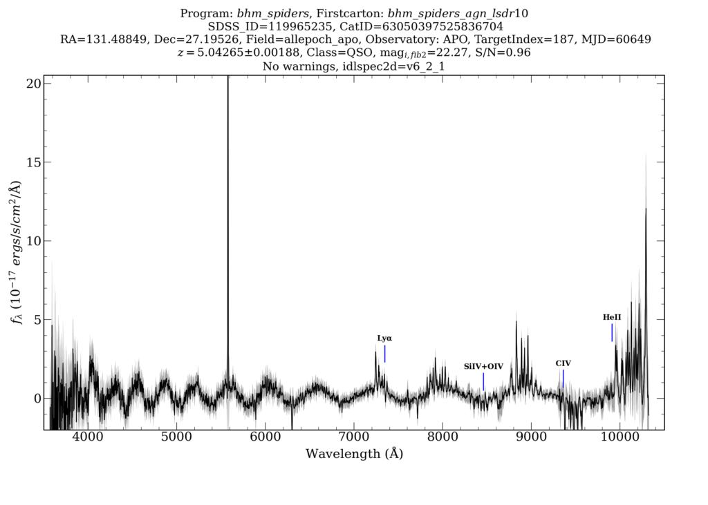
An example of a spectrum showing unexpected wiggles. Note that pipeline finds an incorrect redshift of z>5 for this spectrum.
What else might be affecting my spectrum?
Poor sky subtraction
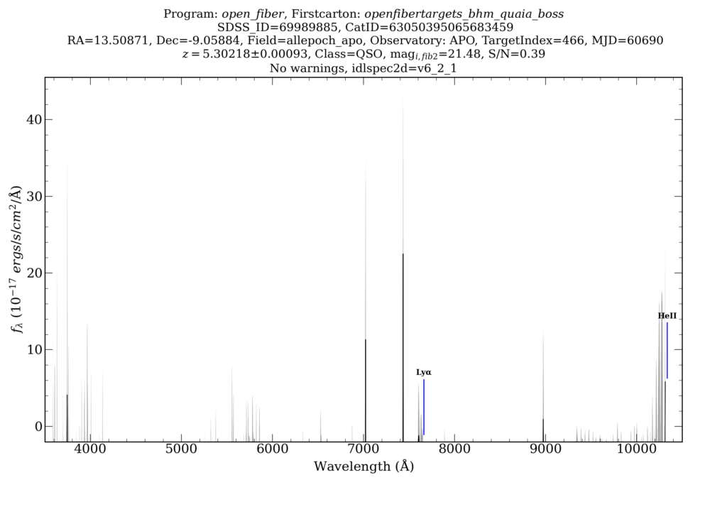
If you have a spectrum dominated by negative pixels, looking like it is underwater, it could be caused by poor sky subtraction.
Poor wavelength calibration
A few fields on particular dates show the skylines at incorrect wavelengths, indicating wavelength calibration issues on certain exposures. See more details in the RV section.